Author Archives: Charles Krebs

On Evolution and Ecology and Climate Change

If ecology can team up with evolution to become a predictive science, we can all profit greatly since it will make us more like physics and the hard sciences. It is highly desirable to have a grand vision of accomplishing this, but there could be a few roadblocks on the way. A recent paper by Bay et al. (2018) illustrates some of the difficulties we face.

The yellow warbler (Setophaga petechia) has a broad breeding range across the United States and Canada, and could therefore be a good species to survey because it inhabits widely different climatic zones. Bay et al. (2018) identified genomic variation associated with climate across the breeding range of this migratory songbird, and concluded that populations requiring the greatest shifts in allele frequencies to keep pace with future climate change have experienced the largest population declines, suggesting that failure to adapt may have already negatively affected population abundance. This study by Bay et al. (2018) sampled 229 yellow warblers from 21 locations across North America, with an average of 10 birds per sample area (range n = 6 to 21). They examined 104,711 single-nucleotide polymorphisms. They correlated genetic structure to 19 climate variables and 3 vegetation indices, a measure of surface moisture, and average elevation. This is an important study claiming to support an important conclusion, and consequently it is also important to break it down into the three major assumptions on which it rests.

First, this study is a space for time analysis, a subject of much discussion already in plant ecology (e.g. Pickett 1989, Blois et al. 2013). It is an untested assumption that you can substitute space for time in analyzing for future evolutionary changes.

Second, the conclusions of the Bay et al. paper rest on an assumption that you have adequate data on the genetics involved in change and on the demography of the species. A clear understanding of the ecology of the species and what limits its distribution and abundance would seem to be prerequisites for understanding the mechanisms of how evolutionary changes might occur.

The third assumption is that, if there is a correlation between the genetic measures and the climate or vegetation indices, one can identify the precise ‘genomic vulnerability’ of the local population. Genomic variation was most closely related to precipitation variables at each site. The geographic area with one of the highest scores in genomic vulnerability was in the desert area of the intermountain west (USA). As far as I can determine from their Figure 1, there was only one sampling site in this whole area of the intermountain west. Finally Bay et al. (2018) compared the genomic vulnerability data to the population changes reported for each site. Population changes for each sampled site were obtained from the North American Breeding Bird Survey data from 1996 to 2012.

The genetic data and its analysis are more impressive, and since I am not a genetics expert I will simply give it a A grade for genetics. It is the ecology that worries me. I doubt that the North American Breeding Bird Survey is a very precise measure of population changes in any particular area. But following the Bay et al. paper, assume that it is a good measure of changing abundance for the yellow warbler. From the Bay et al. paper abstract we see this prediction:

“Populations requiring the greatest shifts in allele frequencies to keep pace with future climate change have experienced the largest population declines, suggesting that failure to adapt may have already negatively affected populations.”

The prediction is illustrated in Figure 1 below from the Bay et al. paper.

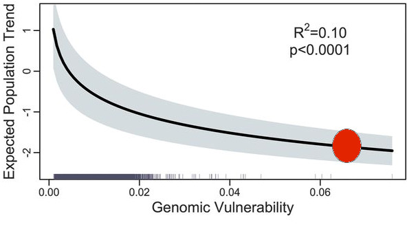
Figure 1. From Bay et al. (2018) Figure 2C. (Red dot explained below).

Consider a single case, the Great Basin, area S09 of the Sauer et al. (2017) breeding bird surveys. From the map in Bay et al. (2018) Figure 2 we get the prediction of a very high genomic vulnerability (above 0.06, approximate red dot in Figure 1 above) for the Great Basin, and thus a strongly declining population trend. But if we go to the Sauer et al. (2017) database, we get this result for the Great Basin (Figure 2 here), a completely stable yellow warbler population for the last 45 years.

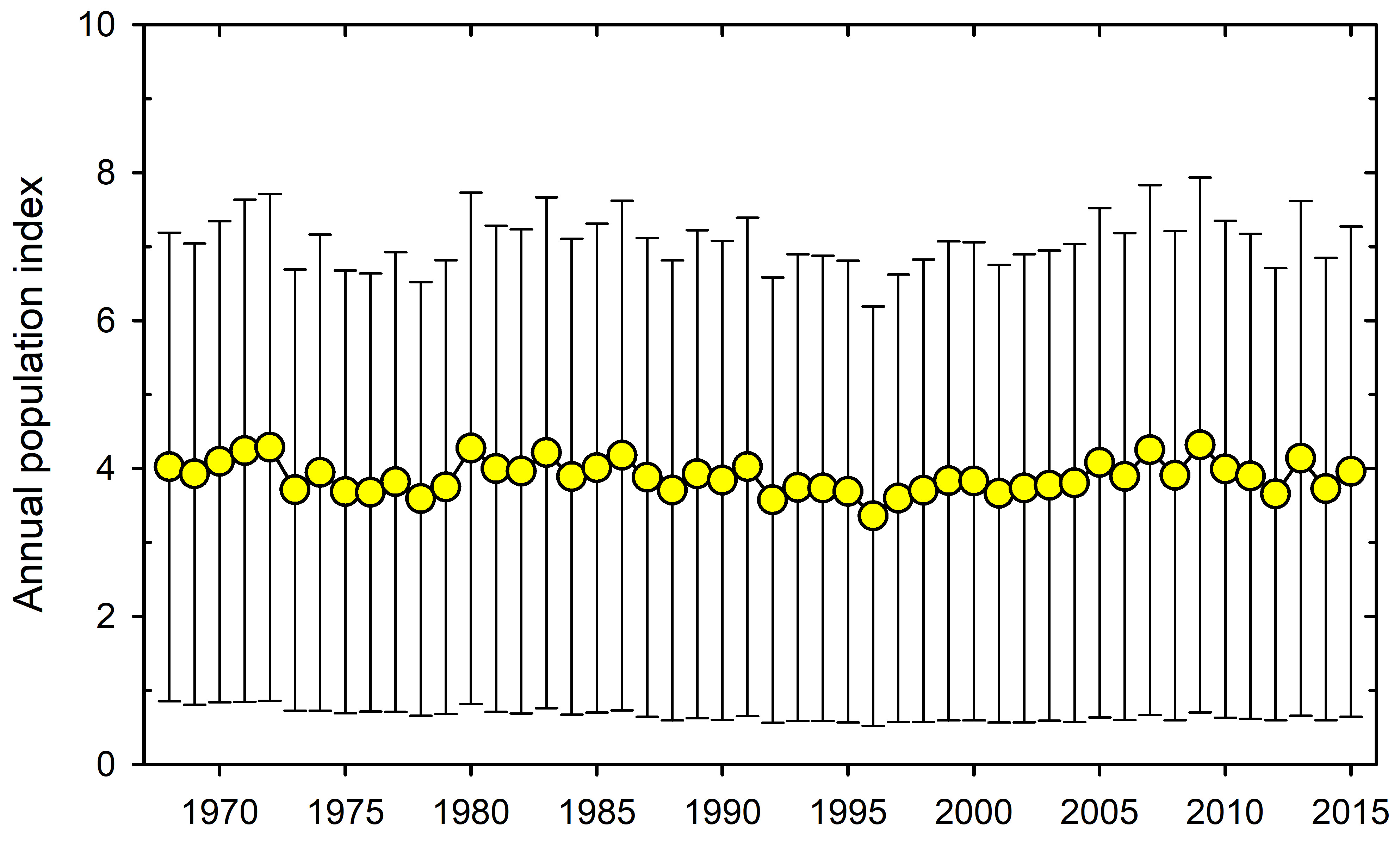
Figure 2. Data for the Great Basin populations of the Yellow Warbler from the North American Breeding Bird Survey, 1967 to 2015 (area S09). (From Sauer et al. 2017)

One clue to this discrepancy is shown in Figure 1 above where R2 = 0.10, which is to say the predictability of this genomic model is near zero.

So where does this leave us? We have what appears to be an A grade genetic analysis coupled with a D- grade ecological model in which explanations are not based on any mechanism of population dynamics, so that the model presented is useless for any predictions that can be tested in the next 10-20 years. I am far from convinced that this is a useful exercise. It would be a good paper for a graduate seminar discussion. Marvelous genetics, very poor ecology.

And as a footnote I note that mammalian ecologists have already taken a different but more insightful approach to this whole problem of climate-driven adaptation (Boutin and Lane 2014).

Bay, R.A., Harrigan, R.J., Underwood, V.L., Gibbs, H.L., Smith, T.B., and Ruegg, K. 2018. Genomic signals of selection predict climate-driven population declines in a migratory bird. Science 359(6371): 83-86. doi: 10.1126/science.aan4380.

Blois, J.L., Williams, J.W., Fitzpatrick, M.C., Jackson, S.T., and Ferrier, S. 2013. Space can substitute for time in predicting climate-change effects on biodiversity. Proceedings of the National Academy of Sciences 110(23): 9374-9379. doi: 10.1073/pnas.1220228110.

Boutin, S., and Lane, J.E. 2014. Climate change and mammals: evolutionary versus plastic responses. Evolutionary Applications 7(1): 29-41. doi: 10.1111/eva.12121.

Pickett, S.T.A. 1989. Space-for-Time substitution as an alternative to long-term studies. In Long-Term Studies in Ecology: Approaches and Alternatives. Edited by G.E. Likens. Springer New York, New York, NY. pp. 110-135.

Sauer, J.R., Niven, D.K., Hines, J.E., D. J. Ziolkowski, J., Pardieck, K.L., and Fallon, J.E. 2017. The North American Breeding Bird Survey, Results and Analysis 1966 – 2015. USGS Patuxent Wildlife Research Center, Laurel, MD. https://www.mbr-pwrc.usgs.gov/bbs/

On the Tasks of Retirement

The end of another year in retirement and time to clean up the office. So this week I recycled 15,000 reprints – my personal library of scientific papers. I would guess that many young scientists would wonder why anyone would have 15,000 paper reprints when you could have all that on a small memory stick. Hence this blog.

Rule #1 of science: read the literature. In 1957 when I began graduate studies there were perhaps 6 journals that you had to read to keep up in terrestrial ecology. Most of them came out 3 or 4 times a year, and if you could not afford to have a personal copy of the paper either by buying the journal or later by xeroxing, you wrote to authors to ask them to post a copy of their paper to you – a reprint. The university even printed special postcards to request reprints with your name and address for the return mail. So scientists gathered paper copies of important papers. Then it became necessary to catalog them, and the simplest thing was to type the title and reference on a 3 by 5-inch card and put them in categories in a file cabinet. All of this will be incomprehensible to modern scientists.

A corollary of this old-style approach to science was that when you published, you had to purchase paper copies of reprints of your own papers. When someone got interested in your research, you would get reprint requests and then had to post them around the world. All this cost money and moreover you had to guess how popular your paper might be in future. The journal usually gave you 25 or 50 free reprints when you published a paper but if you thought you’d need more then you had to purchase them in advance. The first xerox machines were not commercially available until 1959. Xeroxing was quite expensive even when many different types of copying machines started to become available in the late 1960s. But it was always cheaper to buy a reprint when your paper was printed by a journal that it was to xerox a copy of the paper at a later date.

Meanwhile scientists had to write papers and textbooks, so the sorting of references became a major chore for all writers. In 1988 Endnote was first released as a software program that could incorporate references and allow one to sort and print them via a computer, so we were off and running, converting all the 3×5 cards into electronic format. One could then generate a bibliography in a short time and look up forgotten references by author or title or keywords. Through the 1990s the computer world progressed rapidly to approximate what you see today, with computer searches of the literature, and ultimately the ability to download a copy of a PDF of a scientific paper without even telling the author.

But there were two missing elements. All the pre-2000 literature was still piled on Library shelves, and at least in ecology is it possible that some literature published before 2000 might be worth reading. JSTOR (= Journal Storage) came to the rescue in 1995 and began to scan and compile electronic documents of much of this old literature, so even much of the earlier literature became readily available by the early 2000s. Currently there are about 1900 journals in most scientific disciplines that are available in JSTOR. Since by the late 1990s the volume of the scientific literature was doubling about every 7 years, the electronic world saved all of us from yet more paper copies of important papers.

What was missing still were many government and foundation documents, reviews of programs that were never published in the formal literature, now called the ‘grey literature’. Some of these are lost unless governments scan them and make them available. The result of any loss of this grey literature is that studies are sometimes repeated needlessly and money is wasted.

About 2.5 million scientific papers are published every year at the present time (http://www.cdnsciencepub.com/blog/21st-century-science-overload.aspx ) and the consequence of this explosion must be that each of us has to concentrate on a smaller and smaller area of science. What this means for instructors and textbook writers who must synthesize these new contributions is difficult to guess. We need more critical syntheses, but these kinds of papers are not welcomed by those that distribute our research funds so that young scientists feel they should not get caught up in writing an extensive review, however important that is for our science.

In contrast to my feeling of being overwhelmed at the present time, Fanelli and Larivière (2016) concluded that the publication rate of individuals has not changed in the last 100 years. Like most meta-analyses this one is suspicious in arguing against the simple observation in ecology that everyone seems to publish from their thesis many small papers rather than one synthetic one. Anyone who has served on a search committee for university or government jobs in the last 30 years would attest to the fact that the number of publications expected now for new graduates has become quite ridiculous. When I started my postdoc in 1962 I had one published paper, and for my first university job in 1964 this had increased to 3. There were at that time many job opportunities for anyone in my position with a total of 2 or 3 publications. To complicate things, Steen et al. (2013) have suggested that the number of retracted papers in science has been increasing at a faster rate than the number of publications. Whether again this applies to ecology papers is far from clear because the problem in ecology is typically that the methods or experimental design are inadequate rather than fraudulent.

If there is a simple message here, it is that the literature and the potential access to it is changing rapidly and young scientists need to be ready for this. Yet progress in ecology is not a simple metric of counts of papers or even citations. Quality trumps quantity.

Fanelli, D., and Larivière, V. 2016. Researchers’ individual publication rate has not increased in a century. PLoS ONE 11(3): e0149504. doi: 10.1371/journal.pone.0149504.

Steen, R.G., Casadevall, A., and Fang, F.C. 2013. Why has the number of scientific retractions increased?  PLoS ONE 8(7): e68397. doi: 10.1371/journal.pone.0068397.


On Politics and the Environment

This is a short story of a very local event that illustrates far too well the improvements we have to seek in our political systems. The British Columbia government has just approved the continuation of construction of the Site C dam on the Peace River in Northern British Columbia. The project was started in 2015 by the previous Liberal (conservative) government with an $8 billion price tag and with no (yes NO) formal studies of the economic, geological or environmental consequences of the dam, and in complete opposition by most of the First Nations people on whose traditional land the dam would be built. Fast forward 2 years, a moderate left-wing government takes over from the conservatives and the decision is now in their hands: do they carry on with the project, $2 billion having been spent already, or stop it with an additional $1-2 billion in costs to undo the damage to the valley from work already carried out? 2000 temporary construction jobs in the balance, the government in general pro-union and pro the working person rather than the 1%. They decided to proceed with the dam.

To the government’s credit it asked the Utilities Commission to prepare an economic analysis of the project in a very short time, but to make it simpler (?) did not allow the Commission to consider in its report environmental damage, climate change implications, greenhouse gas emissions, First Nations rights, or the loss of good agricultural land. Alas, that pretty well leaves out most things an ecologist would worry about. The economic analysis was sitting on the fence mostly because the question of the final cost of Site C is an unknown. It was estimated to be $8 billion, but already a few days after the government’s decision it is $10.5 billion, all to be paid by the taxpayer. If it is a typical large dam, the final overall cost will range between $16 to $20 billion when the dam is operational in 2024. The best news article I have seen on the Site C decision is this one by Andrew Nikiforuk:

https://thetyee.ca/Opinion/2017/12/12/Pathology-Site-C/

Ansar et al. (2014) did a statistical analysis of 245 large dams built since 1934 and found that on average actual costs for large dams were about twice estimated costs, and that there was a tendency for larger dams to have even higher than average final costs. There has been little study for Site C of the effects of the proposed dam on fish in the river (Cooper et al. 2017) and no discussion of potential greenhouse gas emissions (methane) released as a result of a dam at Site C (DelSontro et al. 2016). The most disturbing comment on this decision to proceed with Site C was made by the Premier of B.C. who stated that if they had stopped construction of the dam, they would have to spend a lot of money “for nothing” meaning that restoring the site, partially restoring the forested parts of the valley, repairing the disturbance of the agricultural land in the valley, recognizing the rights of First Nations people to their land, and leaving the biodiversity of these sites to repair itself would all be classed as “nothing” of value. Alas our government’s values are completely out of line with the needs of a sustainable earth ecosystem for all to enjoy.

What we are lacking, and governments of both stripes have no time for, is an analysis of what the alternatives are in terms of renewable energy generation. Alternative hypotheses should be useful in politics as they are in science. And they might even save money.

Ansar A, Flyvbjerg B, Budzier A, Lunn D (2014). Should we build more large dams? The actual costs of hydropower megaproject development. Energy Policy 69, 43-56. doi: 10.1016/j.enpol.2013.10.069

Cooper AR, et al. (2017). Assessment of dam effects on streams and fish assemblages of the conterminous USA. Science of The Total Environment 586, 879-89. doi: 10.1016/j.scitotenv.2017.02.067

DelSontro T, Perez KK, Sollberger S, Wehrli B (2016). Methane dynamics downstream of a temperate run-of-the-river reservoir. Limnology and Oceanography 61, S188-S203. doi: 10.1002/lno.10387


12 Publishing Mistakes to Avoid

Graduate students probably feel they are given too much advice on their career goals, but it might be useful to list a few of the mistakes I see often while reviewing papers submitted for publication. Think of it as a cheat sheet to go over before final submission of a paper.

  1. Abstract. Write this first and under the realization that 95% of readers will only read this part of your paper. They need in a concise fashion the whole story, particularly for any data paper WHAT, WHERE, WHEN, HOW and WHY.
  2. Graphics. Choose your graphics carefully. Show them to others to see if they get the point immediately. Label the axes carefully. ‘Population’ could mean population size, population density, population index, or something else. ‘Species diversity’ could mean anything from the vast array of species diversity measures.
  3. Precision. If you are plotting data, a single point on a graph is not very informative without some measure of statistical precision. Dot plots without a measure of precision are fraudulent. Indicate at least in the figure legend what exact measure of precision you have used.
  4. Colour and Symbol Shape. If you have 2 or more sets of data, use colour and different symbol shapes to distinguish them. Check that the size of symbols is adequate for the reductions they will use in the journal printing. Journals that charge for colour will often print in black and white for free but use the colour in the PDF version.
  5. Histograms. Use histograms freely in your papers by only after reading Cleveland (1994) who recommends never using histograms. More comments are given in my blog ” On Graphics in Ecological Presentations”.
  6. Scale of Graph. if you wish to cheat there are some simple ways of making your data look better. See Cleveland et al. (1986) for a scatter-plot example.
  7. Tables. Tables should be simple if possible. Columns of meaningless numbers do not help the reader understand your conclusions. Most people understand graphs very quickly but tables very slowly.
  8. Discussion. Be your own critic lest your reviewers do this job for you. If some published papers reach conclusions other than you have, discuss why this might be the case. Recognize that no one study is perfect. Indicate where future research might go.
  9. Literature Cited. Check that all your literature cited in the paper are in the bibliography and none are missed. Check the required format of the references since many editors go into orbit if you use the wrong format or fail to include the doi.
  10. Supplementary Material. Consider carefully what you put in supplementary material. Standards are changing and simple excel tables of mean values are often not enough to be useful for additional analysis.
  11. Covering Letter. A last minute but critical piece of the puzzle because you need to capture in a few sentences why the editor should have your paper reviewed or decide to send it right back to you as not of interest. Remember that editors are swamped with papers and rejection rates are often 60-90% at the first cut.
  12. Select the Right Journal. This is perhaps the hardest part. Not everything in ecology can be published in Science or Nature, and given the electronic world of the Web of Science, good work will be picked up in other journals. If you have millions, you can use the journals that you must pay to publish in, but I personally think this is capitalism gone amok. Romesburg (2016, 2017) presents critical data on the issue of commercial journals in science. Read these papers and put them on your Facebook site.


Cleveland, W.S., Diaconis, P. & McGill, R. (1982) Variables on scatterplots look more highly correlated when the scales are increased. Science, 216, 1138-1141. http://www.jstor.org/stable/1689316

Cleveland, W.S. (1994) The Elements of Graphing Data. AT&T Bell Laboratories, Murray Hill, New Jersey. ISBN: 9780963488411

Romesburg, H.C. (2016) How publishing in open access journals threatens science and what we can do about it. Journal of Wildlife Management, 80, 1145-1151. doi: 10.1002/jwmg.21111

Romesburg, H.C. (2017) How open access is crucial to the future of science: A reply. Journal of Wildlife Management, 81, 567-571. doi: 10.1002/jwmg.21244


On Mauna Loa and Long-Term Studies

If there is one important element missing in many of our current ecological paradigms it is long-term studies. This observation boils down to the lack of proper controls for our observations. If we do not know the background of our data sets, we lack critical perspective on how to interpret short-term studies. We should have learned this from paleoecologists whose many studies of plant pollen profiles and other time series from the geological record show that models of stability which occupy most of the superstructure of ecological theory are not very useful for understanding what is happening in the real world today.

All of this got me wondering what it might have been like for Charles Keeling when he began to measure CO2 levels on Mauna Loa in Hawaii in 1958. Let us do a thought experiment and suggest that he was at that time a typical postgraduate students told by his professors to get his research done in 4 or at most 5 years and write his thesis. These would be the basic data he got if he was restricted to this framework:

Keeling would have had an interesting seasonal pattern of change that could be discussed and lead to the recommendation of having more CO2 monitoring stations around the world. And he might have thought that CO2 levels were increasing slightly but this trend would not be statistically significant, especially if he has been cut off after 4 years of work. In fact the US government closed the Mauna Loa observatory in 1964 to save money, but fortunately Keeling’s program was rescued after a few months of closure (Harris 2010).

Charles Keeling could in fact be a “patron saint” for aspiring ecology graduate students. In 1957 as a postdoc he worked on developing the best way to measure CO2 in the air by the use of an infrared gas analyzer, and in 1958 he had one of these instruments installed at the top of Mauna Loa in Hawaii (3394 m, 11,135 ft) to measure pristine air. By that time he had 3 published papers (Marx et al. 2017). By 1970 at age 42 his publication list had increased to a total of 22 papers and an accumulated total of about 50 citations to his research papers. It was not until 1995 that his citation rate began to exceed 100 citations per year, and after 1995 at age 67 his citation rate increased very much. So, if we can do a thought experiment, in the modern era he could never even apply for a postdoctoral fellowship, much less a permanent job. Marx et al. (2017) have an interesting discussion of why Keeling was undercited and unappreciated for so long on what is now considered one of the world’s most critical environmental issues.

What is the message for mere mortals? For postgraduate students, do not judge the importance of your research by its citation rate. Worry about your measurement methods. Do not conclude too much from short-term studies. For professors, let your bright students loose with guidance but without being a dictator. For granting committees and appointment committees, do not be fooled into thinking that citation rates are a sure metric of excellence. For theoretical ecologists, be concerned about the precision and accuracy of the data you build models about. And for everyone, be aware that good science was carried out before the year 2000.

And CO2 levels yesterday were 407 ppm while Nero is still fiddling.

Harris, D.C. (2010) Charles David Keeling and the story of atmospheric CO2 measurements. Analytical Chemistry, 82, 7865-7870. doi: 10.1021/ac1001492

Marx, W., Haunschild, R., French, B. & Bornmann, L. (2017) Slow reception and under-citedness in climate change research: A case study of Charles David Keeling, discoverer of the risk of global warming. Scientometrics, 112, 1079-1092. doi: 10.1007/s11192-017-2405-z

On Caribou and Hypothesis Testing

Mountain caribou populations in western Canada have been declining for the past 10-20 years and concern has mounted to the point where extinction of many populations could be imminent, and the Canadian federal government is asking why this has occurred. This conservation issue has supported a host of field studies to determine what the threatening processes are and what we can do about them. A recent excellent summary of experimental studies in British Columbia (Serrouya et al. 2017) has stimulated me to examine this caribou crisis as an illustration of the art of hypothesis testing in field ecology. We teach all our students to specify hypotheses and alternative hypotheses as the first step to solving problems in population ecology, so here is a good example to start with.

From the abstract of this paper, here is a statement of the problem and the major hypothesis:

“The expansion of moose into southern British Columbia caused the decline and extirpation of woodland caribou due to their shared predators, a process commonly referred to as apparent competition. Using an adaptive management experiment, we tested the hypothesis that reducing moose to historic levels would reduce apparent competition and therefore recover caribou populations. “

So the first observation we might make is that much is left out of this approach to the problem. Populations can decline because of habitat loss, food shortage, excessive hunting, predation, parasitism, disease, severe weather, or inbreeding depression. In this case much background research has narrowed the field to focus on predation as a major limitation, so we can begin our search by focusing on the predation factor (review in Boutin and Merrill 2016). In particular Serrouya et al. (2017) focused their studies on the nexus of moose, wolves, and caribou and the supposition that wolves feed preferentially on moose and only secondarily on caribou, so that if moose numbers are lower, wolf numbers will be lower and incidental kills of caribou will be reduced. So they proposed two very specific hypotheses – that wolves are limited by moose abundance, and that caribou are limited by wolf predation. The experiment proposed and carried out was relatively simple in concept: kill moose by allowing more hunting in certain areas and measure the changes in wolf numbers and caribou numbers.

The experimental area contained 3 small herds of caribou (50 to 150) and the unmanipulated area contained 2 herds (20 and 120 animals) when the study began in 2003. The extended hunting worked well, and moose in the experimental area were reduced from about 1600 animals down to about 500 over the period from 2003 to 2014. Wolf numbers in the experimental area declined by about half over the experimental period because of dispersal out of the area and some starvation within the area. So the two necessary conditions of the experiment were satisfied – moose numbers declined by about two-thirds from additional hunting and wolf numbers declined by about half on the experimental area. But the caribou population on the experimental area showed mixed results with one population showing a slight increase in numbers but the other two showing a slight loss. On the unmanipulated area both caribou populations showed a continuing slow decline. On the positive side the survival rate of adult caribou was higher on the experimental area, suggesting that the treatment hypothesis was correct.

From the viewpoint of caribou conservation, the experiment failed to change the caribou population from continuous slow declines to the rapid increase needed to recover these populations to their former greater abundance. At best it could be argued that this particular experiment slowed the rate of caribou decline. Why might this be? We can make a list of possibilities:

  1. Moose numbers on the experimental area were not reduced enough (to 300 instead of to 500 achieved). Lower moose would have meant much lower wolf numbers.
  2. Small caribou populations are nearly impossible to recover because of chance events that affect small numbers. A few wolves or bears or cougars could be making all the difference to populations numbering 10-20 individuals.
  3. The experimental area and the unmanipulated area were not assigned treatments at random. This would mean to a pure statistician that you cannot make statistical comparisons between these two areas.
  4. The general hypothesis being tested is wrong, and predation by wolves is not the major limiting factor to mountain caribou populations. Many factors are involved in caribou declines and we cannot determine what they are because they change for area to area, year to year.
  5. It is impossible to do these landscape experiments because for large landscapes it is impossible to find 2 or more areas that can be considered replicates.
  6. The experimental manipulation was not carried out long enough. Ten years of manipulation is not long for caribou who have a generation time of 15-25 years.

Let us evaluate these 6 points.

#1 is fair enough, hard to achieve a population of moose this low but possible in a second experiment.

#2 is a worry because it is difficult to deal experimentally with small populations, but we have to take the populations as a given at the time we do a manipulation.

#3 is true if you are a purist but is silly in the real world where treatments can never be assigned at random in landscape experiments.

#4 is a concern and it would be nice to include bears and other predators in the studies but there is a limit to people and money. Almost all previous studies in mountain caribou declines have pointed the finger at wolves so it is only reasonable to start with this idea. The multiple factor idea is hopeless to investigate or indeed even to study without infinite time and resources.

#5 is like #3 and it is an impossible constraint on field studies. It is a common statistical fallacy to assume that replicates must be identical in every conceivable way. If this were true, no one could do any science, lab or field.

#6 is correct but was impossible in this case because the management agencies forced this study to end in 2014 so that they could conduct another different experiment. There is always a problem deciding how long a study is sufficient, and the universal problem is that the scientists or (more likely) the money and the landscape managers run out of energy if the time exceeds about 10 years or more. The result is that one must qualify the conclusions to state that this is what happened in the 10 years available for study.

This study involved a heroic amount of field work over 10 years, and is a landmark in showing what needs to be done and the scale involved. It is a far cry from sitting at a computer designing the perfect field experiment on a theoretical landscape to actually carrying out the field work to get the data summarized in this paper. The next step is to continue to monitor some of these small caribou populations, the wolves and moose to determine how this food chain continues to adjust to changes in prey levels. The next experiment needed is not yet clear, and the eternal problem is to find the high levels of funding needed to study both predators and prey in any ecosystem in the detail needed to understand why prey numbers change. Perhaps a study of all the major predators – wolves, bears, cougars – in this system should be next. We now have the radio telemetry advances that allow satellite locations, activity levels, timing of mortality, proximity sensors when predators are near their prey, and even video and sound recording so that more details of predation events can be recorded. But all this costs money that is not yet here because governments and people have other priorities and value the natural world rather less than we ecologists would prefer. There is not yet a Nobel Prize for ecological field research, and yet here is a study on an iconic Canadian species that would be high up in the running.

What would I add to this paper? My curiosity would be satisfied by the number of person-years and the budget needed to collect and analyze these results. These statistics should be on every scientific paper. And perhaps a discussion of what to do next. In much of ecology these kinds of discussions are done informally over coffee and students who want to know how science works would benefit from listening to how these informal discussions evolve. Ecology is far from simple. Physics and chemistry are simple, genetics is simple, and ecology is really a difficult science.

Boutin, S. and Merrill, E. 2016. A review of population-based management of Southern Mountain caribou in BC. {Unpublished review available at: http://cmiae.org/wp-content/uploads/Mountain-Caribou-review-final.pdf

Serrouya, R., McLellan, B.N., van Oort, H., Mowat, G., and Boutin, S. 2017. Experimental moose reduction lowers wolf density and stops decline of endangered caribou. PeerJ  5: e3736. doi: 10.7717/peerj.3736.


On Immigration – An Ecological Perspective

There is a great deal of discussion in the news about immigration into developed countries like Canada, USA, and Europe. The perspective on this important issue in the media is virtually entirely economic and social, occasionally moral, but in my experience almost never ecological. There are two main aspects of immigration that are particularly ecological – defining sustainable populations and protecting ecosystems from biodiversity loss. These ecological concerns ought to be part of the discussion.

Sustainability is one of the sciences current buzz words. As I write this, in the Web of Science Core Collection I can find 9218 scientific papers published already in 2017 that appear under the topic of ‘sustainability’. No one could read all these, and the general problem with buzz words like ‘sustainability’ is that they tend to be used so loosely that they verge on the meaningless. Sustainability is critical in this century, but as scientists we must specify the details of how this or that public policy really does increase some metric of sustainability.

There have been several attempts to define what a sustainable human population might be for any country or the whole Earth (e.g. Ehrlich 1996, Rees and Wackernagel 2013) and many papers on specific aspects of sustainability (e.g. Hilborn et al. 2015, Delonge et al. 2016). The controversy arises in specifying the metric of sustainability. The result is that there is no agreement particularly among economists and politicians about what to target. For the most part we can all agree that exponential population growth cannot continue indefinitely. But when do we quit? In developed countries the birth rate is about at equilibrium, and population growth is achieved in large part by immigration. Long term goals of achieving a defined sustainable population will always be trumped in the short term by changes in the goal posts – long term thinking seems almost impossible in our current political systems. One elephant in the room is that what we might define now as sustainable agriculture or sustainable fisheries will likely not be sustainable as climates change. Optimists predict that technological advances will greatly relieve the current limiting factors so all will be well as populations increase. It would seem to be conservative to slow our population growth, and thus wait to see if this optimism is justified (Ehrlich and Ehrlich 2013).

Few developed countries seem to have set a sustainable population limit. It is nearly impossible to even suggest doing this, so this ecological topic disappears in the media. One possible way around this is to divert the discussion to protecting ecosystems from biodiversity loss. This approach to the overall problem might be an easier topic to sell to the public and to politicians because it avoids the direct message about population growth. But too often we run into a brick wall of economics even when we try this approach to sustainability because we need jobs for a growing population and the holy grail of continued economic growth is a firm government policy almost everywhere (Cafaro 2014, Martin et al. 2016). At present this biodiversity approach seems to be the best chance of convincing the general public and politicians that action is needed on conservation issues in the broad sense. And by doing this we can hopefully obtain action on the population issue that is blocked so often by political and religious groups.

A more purely scientific issue is the question why the concept of a sustainable population is thought to be off limits for a symposium at a scientific meeting? In recent years attempts to organize symposia on sustainable population concepts at scientific conferences have been denied by the organizers because the topic is not considered a scientific issue. Many ecologists would deny this because without a sustainable population, however that is defined, we may well face social collapse (Ehrlich and Ehrlich 2013).

What can we do as ecologists? I think shying away from these population issues is impossible because we need to have a good grounding in population arithmetic to understand the consequences of short-term policies. It is not the ecologist’s job to determine public policy but it is our job to question much of the pseudo-scientific nonsense that gets repeated in the media every day. At least we should get the arithmetic right.

Cafaro, P. (2014) How Many Is Too Many? The Progressive Argument for Reducing Immigration into the United States. University of Chicago Press, Chicago. ISBN: 9780226190655

DeLonge, M.S., Miles, A. & Carlisle, L. (2016) Investing in the transition to sustainable agriculture. Environmental Science & Policy, 55, 266-273. doi: 10.1016/j.envsci.2015.09.013

Ehrlich, A.H. (1996) Towards a sustainable global population. Building Sustainable Societies (ed. D.C. Pirages), pp. 151-165. M. E. Sharpe, London. ISBN: 1-56324-738-0, 978-1-56324-738-5

Ehrlich, P.R. & Ehrlich, A.H. (2013) Can a collapse of global civilization be avoided? Proceedings of the Royal Society B: Biological Sciences, 280, 20122845. doi: 10.1098/rspb.2012.2845

Hilborn, R., Fulton, E.A., Green, B.S., Hartmann, K. & Tracey, S.R. (2015) When is a fishery sustainable? Canadian Journal of Fisheries and Aquatic Sciences, 72, 1433-1441. doi: 10.1139/cjfas-2015-0062

Hurlbert, S.H. (2013) Critical need for modification of U.S. population policy. Conservation Biology, 27, 887-889. doi: 10.1111/cobi.12091

Martin, J.-L., Maris, V. & Simberloff, D.S. (2016) The need to respect nature and its limits challenges society and conservation science. Proceedings of the National Academy of Sciences, 113, 6105-6112. doi: 10.1073/pnas.1525003113

Rees W.E. &, Wackernagel, M. (2013). The shoe fits, but the footprint is larger than Earth. PLOS Biology 11, e1001701. doi: 10.1371/journal.pbio.1001701

On Defining a Statistical Population

The more I do “field ecology” the more I wonder about our standard statistical advice to young ecologists to “random sample your statistical population”. Go to the literature and look for papers on “random environmental fluctuations”, or “non-random processes”, or “random mating” and you will be overwhelmed with references and biology’s preoccupation with randomness. Perhaps we should start with the opposite paradigm, that nothing in the biological world is random in space or time, and then the corollary that if your data show a random pattern or random mating or whatever random, it means you have not done enough research and your inferences are weak.

Since virtually all modern statistical inference rests on a foundation of random sampling, every statistician will be outraged by any concerns that random sampling is possible only in situations that are scientifically uninteresting. It is nearly impossible to find an ecological paper about anything in the real world that even mentions what their statistical “population” is, what they are trying to draw inferences about. And there is a very good reason for this – it is quite impossible to define any statistical population except for those of trivial interest. Suppose we wish to measure the heights of the male 12-year-olds that go to school in Minneapolis in 2017. You can certainly do this, and select a random sample, as all statisticians would recommend. And if you continued to do this for 50 years, you would have a lot of data but no understanding of any growth changes in 12-year-old male humans because the children of 2067 in Minneapolis would be different in many ways from those of today. And so, it is like the daily report of the stock market, lots of numbers with no understanding of processes.

Despite all these ‘philosophical’ issues, ecologists carry on and try to get around this by sampling a small area that is considered homogeneous (to the human eye at least) and then arm waving that their conclusions will apply across the world for similar small areas of some ill-defined habitat (Krebs 2010). Climate change may of course disrupt our conclusions, but perhaps this is all we can do.

Alternatively, we can retreat to the minimalist position and argue that we are drawing no general conclusions but only describing the state of this small piece of real estate in 2017. But alas this is not what science is supposed to be about. We are supposed to reach general conclusions and even general laws with some predictive power. Should biologists just give up pretending they are scientists? That would not be good for our image, but on the other hand to say that the laws of ecology have changed because the climate is changing is not comforting to our political masters. Imagine the outcry if the laws of physics changed over time, so that for example in 25years it might be that CO2 is not a greenhouse gas. Impossible.

These considerations should make ecologists and other biologists very humble, but in fact this cannot be because the media would not approve and money for research would never flow into biology. Humility is a lost virtue in many western cultures, and particularly in ecology we leap from bandwagon to bandwagon to avoid the judgement that our research is limited in application to undefined statistical populations.

One solution to the dilemma of the impossibility of random sampling is just to ignore this requirement, and this approach seems to be the most common solution implicit in ecology papers. Rabe et al. (2002) surveyed the methods used by management agencies to survey population of large mammals and found that even when it was possible to use randomized counts on survey areas, most states used non-random sampling which leads to possible bias in estimates even in aerial surveys. They pointed out that ground surveys of big game were even more likely to provide data based on non-random sampling simply because most of the survey area is very difficult to access on foot. The general problem is that inference is limited in all these wildlife surveys and we do not know the ‘population’ to which the numbers derived are applicable.

In an interesting paper that could apply directly to ecology papers, Williamson (2003) analyzed research papers in a nursing journal to ask if random sampling was utilized in contrast to convenience sampling. He found that only 32% of the 89 studies he reviewed used random sampling. I suspect that this kind of result would apply to much of medical research now, and it might be useful to repeat his kind of analysis with a current ecology journal. He did not consider the even more difficult issue of exactly what statistical population is specified in particular medical studies.

I would recommend that you should put a red flag up when you read “random” in an ecology paper and try to determine how exactly the term is used. But carry on with your research because:

Errors using inadequate data are much less than those using no data at all.

Charles Babbage (1792–1871

Krebs CJ (2010). Case studies and ecological understanding. Chapter 13 in: Billick I, Price MV, eds. The Ecology of Place: Contributions of Place-Based Research to Ecological Understanding. University of Chicago Press, Chicago, pp. 283-302. ISBN: 9780226050430

Rabe, M. J., Rosenstock, S. S. & deVos, J. C. (2002) Review of big-game survey methods used by wildlife agencies of the western United States. Wildlife Society Bulletin, 30, 46-52.

Williamson, G. R. (2003) Misrepresenting random sampling? A systematic review of research papers in the Journal of Advanced Nursing. Journal of Advanced Nursing, 44, 278-288. doi: 10.1046/j.1365-2648.2003.02803.x


Fire and Fury and the Environment

The media at present is full of comments about having a war that will stimulate the economy, at least in reconstruction. And this concern over war and the costs of war prompted me to investigate the relative costs of military funding and environmental funding. So here is a very coarse look at the relative positions of military funding and environmental funding in a few western countries. All the numbers are approximate and refer to 2016 and possibly 2017 budgets, and all are in billions of dollars.

Military expenditures by countries are easiest to obtain, and here are a few for the most recent years I could find:

United States:         $ 611 billion
China:                       $ 216
Russia:                      $ 69
Saudi Arabia:           $ 64
Australia:                  $ 24
Canada:                    $ 15.5

Environmental funding is much more difficult to decompose because different countries amalgamate different agencies into one Department. Consequently, comparisons are best made within one country rather than between countries. Here are a few details for particular agencies:

USA            Department of the Interior     $ 13.4            1 military year = 46 Dept. years
NOAA                                                             $ 5.77             1 military year = 106 NOAA years

Canada      Environment Canada              $ 0.987            1 military year = 16 EC years

Australia     CSIRO                                       $ 0.803            1 military year = 30 CSIRO years

Clearly there are many problems with these simple comparisons. NOAA for example includes agencies covering Marine Fisheries, Weather Service, Environmental Satellites, Aviation Operations, and Oceanic Research among other responsibilities. CSIRO includes divisions dealing with agriculture, climate change, and mining research. I am sure that someone has done a more detailed analysis of these comparisons, but the general message is very clear: the environment is a low priority among western nations, and if you want a rough number one might say the military is about 30 times more “important” than the environment when it comes to funding. If you look for example at the Australian budget for 2017 (http://budget.gov.au/2017-18/content/glossies/overview/download/Budget2017-18-Overview.pdf ) and search for the word ‘environment’ as in the real biophysical environment, you will find not a single case of this word appearing. It is as though the biophysical environment does not exist as a problem in 2017.

I am not clear if anyone worries about these simple facts. The general problem is that federal government budgets are made so complex and presented so poorly that it is nearly impossible to separate out different equivalent expenditures. Thus for example the military argues that it does scientific research with part of its funding, and universities fail to point out that some of their basic research focuses on military questions rather than questions that might benefit humanity (Smart 2016).

I hope that others might look into these expenditures in more detail, and that in the long run we might be more aware of where our tax dollars go. The simple suggestion that the last page of our tax file should give us a choice of what general areas we would like to support with our taxes would be a start. On the last list I saw of 25 ‘items of interest’ to taxpayers who might like more information, the words ‘environment’, ‘conservation’, or ‘sustainability’ never appeared. We should demand this be changed.
Smart, B. (2016). Military-industrial complexities, university research and neoliberal economy. Journal of Sociology 52, 455-481. doi: 10.1177/1440783316654258

On Ecology and Economics

Economics has always been a mystery to me, so if you are an economist you may not like this blog. Many ecologists and some economists have written elegantly about the need for a new economics that includes the biosphere and indeed the whole world rather than just Wall Street and brings together ecology and the social sciences (e.g. Daily et al. 1991, Haly and Farley 2011, Brown et al. 2014, Martin et al. 2016). Several scientists have proposed measures that indicate how our current usage of natural resources is unsustainable (Wackernagel and Rees 1996, Rees and Wackernagel 2013). But few influential people and politicians appear to be listening, or if they are listening they are proceeding at a glacial pace at the same time as the problems that have been pointed out are racing at breakneck speed. The operating paradigm seems to be ‘let the next generation figure it out’ or more cynically ‘we are too busy buying more guns to worry about the environment’.

Let me discuss Canada as a model system from the point of view of an ecologist who thinks sustainability is something for the here and now. Start with a general law. No country can base its economy on non-renewable resources. Canada subsists by mining coal, oil, natural gas, and metals that are non-renewable. It also makes ends meet by logging and agricultural production. And we have done well for the last 200 years doing just that. Continue on, and to hell with the grandkids seems to be the prevailing view of the moment. Of course this is ecological nonsense, and, as many have pointed out, not the path to a sustainable society. Even Canada’s sustainable industries are unsustainable. Forestry in Canada is a mining operation in many places with the continuing need to log old growth forest to be a viable industry. Agriculture is not sustainable if soil fertility is continually falling so that there is an ever-increasing need for more fertilizer, and if more agricultural land is being destroyed by erosion and shopping malls. All these industries persist because of a variety of skillful proponents who dismiss long-term problems of sustainability. The oil sands of Alberta are a textbook case of a non-renewable resource industry that makes a lot of money while destroying both the Earth itself and the climate. Again, this makes sense short-term, but not for the grandkids.

So, we see a variety of decisions that are great in the short term but a disaster in the long term. Politicians will not move now unless the people lead them and there is little courage shown and only slight discussion of the long-term issues. The net result is that it is most difficult now to be an ecologist and be optimistic of the future even for relatively rich countries. Global problems deserve global solutions yet we must start with local actions and hope that they become global. We push ahead but in every case we run into the roadblocks of exponential growth. We need jobs, we need food and water and a clean atmosphere, but how do we get from A to B when the captains of industry and the public at large have a focus on short-term results? As scientists we must push on toward a sustainable future and continue to remind those who will listen that the present lack of action is not a wise choice for our grandchildren.

Brown, J.H. et al. 2014. Macroecology meets macroeconomics: Resource scarcity and global sustainability. Ecological Engineering 65(1): 24-32. doi: 10.1016/j.ecoleng.2013.07.071.

Daily, G.C., Ehrlich, P.R., Mooney, H.A., and Erhlich, A.H. 1991. Greenhouse economics: learn before you leap. Ecological Economics 4: 1-10.

Daly, H.E., and Farley, J. 2011. Ecological Economics: Principles and Applications. 2nd ed. Island Press, Washington, D.C.

Martin, J.-L., Maris, V., and Simberloff, D.S. 2016. The need to respect nature and its limits challenges society and conservation science. Proceedings of the National Academy of Sciences 113(22): 6105-6112. doi: 10.1073/pnas.1525003113.

Rees, W. E., and M. Wackernagel. 2013. The shoe fits, but the footprint is larger than Earth. PLoS Biology 11:e1001701. doi: 10.1371/journal.pbio.1001701

Wackernagel, M., and W. E. Rees. 1996. Our Ecological Footprint: Reducing Human Impact on the Earth. New Society Publishers, Gabriola Island, B.C. 160 p.