Biology 301

Non-Linear Equations

We now turn our attention to models that describe the dynamics of a system in terms of NON-LINEAR equations in more than one variable.

With occasional exceptions, non-linear systems of equations do not yield general solutions (i.e. they are often intractable).

Other methods of analysing equations therefore become especially important, including

graphical analyses
identification of equilibria
stability analysis of the equilibria

We will focus on two examples of non-linear systems of equations:

Lotka-Volterra model of competition
Spread of disease through a population

Lotka-Volterra Model of Competition

Species do not exist in isolation of one another. The simple models of exponential and logistic growth fail to capture the fact that species can

compete for resources
assist one another
exclude one another
kill one another

Here we will generalize the logistic model to take into account resource competition between two species.

Model Parameters

Let

= # of individuals of species 2

= intrinsic growth rate of species 1

= intrinsic growth rate of species 2

= carrying capacity of species 1 when species 2 is absent

= carrying capacity of species 2 when species 1 is absent

Lotka-Volterra Model of Competition

The assumption underlying the Lotka-Volterra competition equations is that competing species use of some of the resources available to a species (as if there were actually more individuals of the latter species):

is called the COMPETITION COEFFICIENT measuring the effect of an individual of species 2 on an individual of species 1. Similarly,

Discrete Model

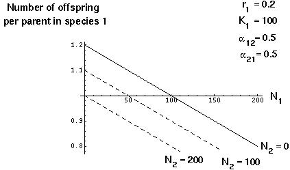
The assumption of the logistic model is that the number of offspring per parent decreases linearly with the number of individuals (of species 1) currently in the population.

With a second competing species also present, the number of offspring per parent depends not only on , but also on the value of :

Lotka-Volterra Model of Competition

Therefore the population size in the next generation will equal:

Similarly,

Continuous Model

In this case, it is assumed that the individual's contribution to the population growth rate is

for species 2

Therefore the growth rate of the entire population is equal to:

for species 2

We'll focus on the discrete case in class.

Lotka-Volterra Model of Competition

Note:

In both the discrete and continuous cases,

If equals zero, then the dynamics of species 1 will follow the logistic equation we analysed before.
If equals zero, then the dynamics of species 2 will follow the logistic equation we analysed before.
If equals one, then individuals of species 2 compete for the resources of species 1 just as strongly as do members of species 1 (interspecific competition is as strong as intraspecific competition).
If is negative, then the presence of species 2 increases the resources available to species 1.

If both and are negative, the species are said to have a mutualistic relationship.

If or is negative and the other is zero (or very nearly zero), the species are said to have a commensal relationship.

If one of the two is positive and one is negative, the species are said to have a parasitic relationship.

If both are positive, the species are said to have a competitive relationship.

We will analyse the effects of competition (with > 0 and > 0) on the dynamics of two species.

Lotka-Volterra Model of Competition

Preliminary Graphical Analysis

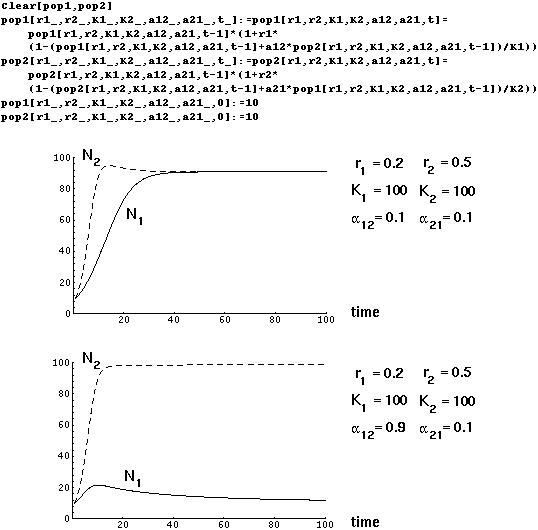
The first step of an analysis might be to graph examples to see what happens to each of the species under different parameter conditions:

When and are small, both species approach an equilibrium level near their carrying capactities. If is much higher than (species 2 impacts more strongly on the resources of species 1 than vice versa), then species 1 will be kept at low numbers by the competitive superiority of species 2.

Lotka-Volterra Model of Competition

Such a graphical method is only useful for specific examples, however, and doesn't give us a general picture of what will happen and when.

Identification of Equilibria

As before, we determine equilibria by finding out when the variables will stay constant over time.

Unlike the case of a single variable and a single function, however, we must find an equilibrium solution where ALL of the variables remain constant over time.

For the continuous model of competition, this requires that d/dt = 0 AND that d/dt = 0.

For the discrete model of competition, this requires that [t+1] = [t] AND that [t+1] = [t].

Setting [t+1] = [t] = in the discrete equation for species 1 gives:

There are two ways in which this equation can be satisfied:

Lotka-Volterra Model of Competition

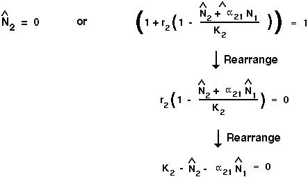
Setting [t+1] = [t] = in the discrete equation for species 2 gives:

Again, there are two ways in which this equation can be satisfied:

At equilibrium, there are four ways to ensure that both and remain constant over time:

both species are extinct ( = 0 and =0)
species 1 is extinct ( = 0 and =)
species 2 is extinct ( = and =0)
both species are present.

Lotka-Volterra Model of Competition

To get both species to persist at equilibrium requires that both

To solve both equations simultaneously:

Solve one equation for in terms of .
Plug this value for into the other equation.
Solve the resulting equation for in terms of the parameters of the model.
Finally, plug this equilibrium value for into one of the above equations to get an equation for .

Only at this point will both species be present in constant numbers over time.

Back to biology 301 home page.