
Bayesian analysis
This workshop will illustrate some of the principles of data analysis in a Bayesian framework. For probability and likelihood calculations consult the probability tab at the R tips help page.Data analysis in a Bayesian framework is related to likelihood methods. An important difference is that Bayesian methods require a prior probability for hypotheses or parameter values. Statistical inference is based on the posterior probability distribution for the hypotheses or parameter values.
Remember that the likelihood is
Likelihood( parameter |
data ) = Pr( data | parameter ).
Bayesian posterior probabilities are based on the likelihoods as follows:
Pr( parameter | data ) = Likelihood ( parameter | data ) x Pr (parameter) /
sum( Likelihood ( parameter_i | data ) x Pr (parameter_i) )
where
- Pr( parameter | data ) = posterior probability of a specific parameter value
- Likelihood ( parameter | data ) = likelihood of that specific parameter value
- Pr (parameter) = prior probability of that specific parameter value
- sum( Likelihood ( parameter_i | data ) x Pr
(parameter_i) ) = sum of the likelihoods of each possible
parameter value multiplied by its prior probability
Elephant population size
This example continues one from an earlier workshop. Eggert et al. (2003. Molecular Ecology 12: 1389–1402) used mark-recapture methods to estimate the total number of forest elephants inhabiting Kakum National Park in Ghana by sampling dung and extracting elephant DNA to uniquely identify individuals. We will review the likelihood estimates for population size and then use Bayesian estimation to generate a credible interval for population size.Over the first seven days of collecting the researchers identified 27 elephant individuals. Refer to these 27 elephants as marked. Over the next eight days they sampled 74 individuals, of which 15 had been previously marked. Refer to these 15 elephants as recaptured.
Provided the assumptions are met (see likelihood workshop), then the number of recaptured (i.e., previously marked) individuals X in the second sample should have a hypergeometric distribution with parameters k (the size of the second sample of individuals), m (total number of marked individuals in the population when the second sample was taken), and n (total number of unmarked individuals in the population when the second sample was taken).
- Using the hypergeometric distribution, calculate the likelihood of each of possible values for the number of elephants in the Park. Note that the total number of elephants is n + m, and that m is known (m = 27). Note also that only integer values for n are allowed, and that n cannot be smaller than k - X, the observed number of unmarked individuals in the second sample.
- Find the value of n that maximizes the likelihood. Add m to this number to obtain the maximum likelihood estimate for population size.
- Calculate the likelihood-based 95% confidence interval for the total number of elephants.
- Decide on a minimum and maximum possible value for n, the number of unmarked elephants in the Park (or n + m, the total number, if that's how you're calculating the likelihoods). The minimum n can be as small as 0 but the likelihood will be 0 for values smaller than k - X, so it is practical to set the smallest n to something greater or equal to k - X. For this first exercise don't set the maximum too high. We'll explore what happens later when we set the maximum to be a very large number.
- Create a vector of n values (or n + m values) containing all the integers between and including the minimum and maximum values that you decided in (4).
- Calculate the likelihoods of each of these values for n. Plot the likelihoods against n. (When calculating these likelihoods, set the option "log=FALSE" because we need the likelihoods rather than the log-likelihoods for the posterior probability calculations.)
- Create a vector containing the prior probabilities for each of the possible values for n that you included in your vector in (5). If you are using a flat prior then the vector will be the same length as your n vector, and each element will be the same constant. Plot the prior probabilities against n. If all is OK at this stage then the plot should show a flat line. Also, confirm that the prior probabilities sum to 1.
- Using your two vectors from (6) and (7), calculate the posterior probabilities of all the possible values of n (or of n + m) between your minimum and maximum values. After your calculation, confirm that the posterior probabilities sum to 1. Plot the posterior probabilities against n (or n + m). Compare with the shape of the likelihood curve.
- What is the most probable value of n + m, given the data? Compare this with your previous maximum likelihood estimate.
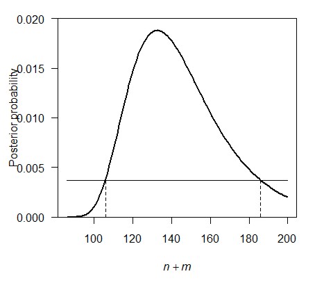
- Calculate the 95% credible interval for n (or n + m,
the total
population size). The procedure for finding the lower and upper limits
of the credible interval is a bit like that for likelihood. The idea is
illustrated in the figure below. Starting from the highest point of the
posterior probability, slide a
horizontal line downward until you reach a point at which the
corresponding values for the parameter (indicated below by the dashed
vertical lines) bracket an area of 0.95 under the curve.
Before reading the instructions in the following sentence, try to think of a method in R to find the values for n (or n + m) that correspond to an are under the curve equal to 0.95.
Here is one way to find the lower and upper limits to the credible interval. Create new vectors containing the posterior probabilities and the parameter values sorted according to the posterior probabilities, starting from the top down:
post.ordered <- posterior[order(posterior,decreasing=TRUE)]
n.ordered <- n[order(posterior,decreasing=TRUE)]
where "n" is the vector containing your possible values of population size, and "posterior" is the vector containing the corresponding posterior probabilities. Next, create a third vector that stores the cumulative ordered probabilities. Finally find the values of n corresponding approximately to a cumulative ordered probability of 0.95.
post.cumsum <- cumsum(post.ordered)
range(n.ordered[post.cumsum <= 0.95])
The area under the curve corresponding to this interval will actually sum to slightly less than 0.95. To adjust, you'll need to subtract 1 from the smallest n in the interval, or add 1 to the largest n in the interval, depending on which corresponding n has the higher posterior probability.
- Compare your 95% credible interval for population size with the approximate likelihood-based 95% confidence interval. Which interval is narrower? Also compare the interpretations of the two intervals. How are they different? Are they compatible? Which makes the most sense to you? Why?
- Repeat the procedures (4)-(10) but using a much larger value for the maximum possible population size. How is your credible interval affected by the increase in the maximum value of the posterior probability distribution?
- What general implication do you draw from the influence of
the
prior probability distribution on the interval estimate for population
size? Do you consider this implication to be a weakness or a strength
of the Bayesian approach?
Biodiversity and ecosystem function
In this second example we will compare the fit of linear and nonlinear models to a data set using a Bayesian model selection criterion. Consult the "fit model" tab of the Rtips pages for information on how to calculate the Bayesian Information Criterion (BIC).We haven't discussed nonlinear model fitting before. Information on how to fit a nonlinear model using "nls" in R is also provided on the "fit models" tab at the Rtips web site.
We will investigate the relationship between an ecosystem function variable, CO2 flux, and the number of eukaryote species (protists and small metazoans) in an experimental aquatic microcosms. (An average of 24 bacterial species was present but not included in the species counts.) The data are from J. McGrady-Steed, P. M. Harris & P. J. Morin (1997, Nature 390: 162-165). Download it from here. The variables are:
- realized number of species, ranging from 2 to 19; may be lower than the number of species initially introduced by the experiments because of extinctions.
- cumulative CO2 flux, a measure of total ecosystem respiration.
Let's consider two hypotheses.
H1: A linear relationship is expected between community respiration and the number of species if each new species added makes the same contribution to ecosystem respiration regardless of how many species are already present.
H2: The second hypothesis is that as the number of species increases, each new species makes a smaller and smaller contribution to ecosystem respiration. This is what we would expect if multi-species communities include species that are functionally redundant, at least for univariate measures of ecosystem function. Under this view, a Michaelis-Menten equation might fit the data because it has an asymptote.
- Download and read the data from the file.
- Plot CO2 flux against number of species.
- Fit a simple linear regression to the data. Add the regression line to the plot. Judging by eye, is it a good fit?
- Fit a Michaelis-Menten model to the data. You'll need to use the version of the formula having a non-zero intercept. (Note: When I tried to fit the model to the data the estimation process did not converge, perhaps because 2 is the smallest value for the explanatory variable -- there are no measurements for 0 and 1 species. I had better luck when I used the number of species minus 2 rather than number of species as the explanatory variable in the model formula). Add the fitted line to the plot. Judging by eye, is it a good fit?
- Calculate BIC for both the linear and nonlinear models that you fit in (3) and (4). Which hypothesis has the lowest BIC? Does this accord with your visual judgements of model fit?
- Calculate the BIC differences for the two models, and then the BIC weights. These weights can be interpreted as Bayesian posterior probabilities of the models if both the linear and Michaelis-Menten models have equal prior probabilities, and if we assume that one of these two models is the "true" model. Of course, we can never know whether either of these models is "true", but we can nevertheless use the weights as a measure of evidence in support of both model, if we are considering only these two.
- Compare the models using AIC instead of BIC. Do you get the same "best" model using this criterion instead?