Population Growth

The abundance of natural populations changes over time in response to:

food and resource availability,
weather conditions,
competition,
predation,
disease...

The simplest models describing changes in population size are exponential growth and logistic growth, which assume

constant food and resource availability,
a constant environment,
no interactions with other species,
no disease

The exponential model also assumes no competition among the members of a species for the available resources (density independent), while the logistic model includes competition within a species for resources (density dependent).

Both of these models can be described by equations in discrete time or continuous time.

Discrete time models are appropriate for organisms with non-overlapping generations such as an annual plant or an insect population with one generation per year.
Continuous time models are appropriate for organisms with overlapping generations in a non-seasonal environment such as microorganisms grown in culture. They are also appropriate for organisms with overlapping generations growing in a seasonal environment if they are censused in the same season, such as perennial plants censused in the spring.

Exponential Growth in Discrete Time

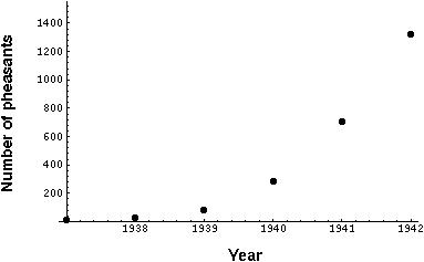
In 1937, two cocks and six hen pheasants were introduced onto an island off the coast of Washington. Over the next five years the population experienced exponential growth (Lack 1954):

The model of exponential growth in discrete time follows from the assumption that each individual will have the same number of offspring on average (R), regardless of the population size.

If there are n[t] individuals in the population at time t, then in the next generation there will be:

n[t+1] = R n[t]

This is the recursion equation describing the change in population size from generation to generation.

Starting at generation 0, there will be R n[0] individuals in the first generation, R² n[0] individuals in the second generation, R³ n[0] individuals in the third generation, and so on.

n[t] = R^t n[0]

This is the general solution giving the population size over time.

Exponential Growth in Continuous Time

The model of exponential growth in continuous time follows from the assumption that each individual reproduces at a constant rate (r), regardless of the population size.

If there are n[t] individuals in the population at time t, then the rate of change of the whole population will be:

dn[t]/dt = r n[t]

This is the differential equation describing the rate of change of the population size.

What is the solution to this differential equation?

n[t] = E^{r t} n[0]

Notice that this general solution is the same as that in discrete time if we define R=E^r.

Also notice that there can be exponential decline in population size if R<1 in the discrete model or r<0 in the continuous model.

Exponential growth cannot, however, continue indefinitely.

Had the pheasants continued to grow exponentially, there would have been 7 million of them by the year 1950 and 10²⁸ by now -- which at 2 kg per pheasant is 3000 times the mass of the earth!!

In fact, Lack observed that "the figures suggest that the increase was slowing down and was about to cease, but at this point the island was occupied by the military and many of the birds shot."

Back to biology 301 home page.