Matrix Algebra

Review: We will briefly review the matrix terms introduced last class, using examples of matrices and vectors in 2-dimensions.

A SCALAR is a constant, variable, or function but not a matrix or vector.

A COLUMN VECTOR has elements arranged one on top of another, e.g.

A ROW VECTOR has elements arranged left to right, e.g.

A MATRIX has multiple rows and columns, e.g.

An IDENTITY MATRIX has ones on the diagonal and zeros elsewhere, e.g.

Vector and matrix ADDITION adds together elements in the same position:

Matrix Algebra

Matrix MULTIPLICATION multiplies the ith row of the first matrix by the jth column in the second matrix and place it in the ij position of the new matrix:

The TRANSPOSE of a matrix makes the rows into columns:

The DETERMINANT of a 2x2 matrix is:

The INVERSE of a 2x2 matrix is:

Matrix Algebra

Review: We will now review the steps outlined in the handout for analysing linear equations.

Step 1: Write the equations in matrix form (an nxn matrix).

Step 2: Determine the n eigenvalues of the matrix.

Step 3: Make a diagonal matrix, D, with one eigenvalue in each of the diagonal positions.

Step 4: Determine the eigenvectors associated with each eigenvalue.

Step 5: Make a transformation matrix, A, whose columns are the eigenvectors (placed in the same order as the eigenvalues in matrix D).

Step 6: Write the general solution of the linear equations as:

This method allows you to say exactly where the system will be at any time in the future.

For example, you can determine what the stable equilibria are by determining where the population will tend as time goes to infinity.

Matrix Algebra

Additional Terms: Here are more matrix terms used in the handout, again with examples in two dimensions.

The EIGENVALUE of a matrix is any scalar () for which a non-zero vector () can be found which solves the equation:

[The eigenvalues are also the roots of the equation Det(J-I)=0, which is how they are usually found.]

The vector () associated with a particular eigenvalue is the EIGENVECTOR.

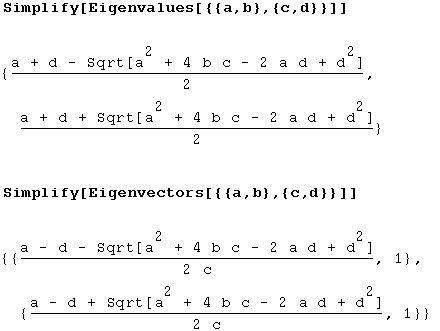
We can use Mathematica to help find eigenvalues and eigenvectors:

Back to biology 301 home page.