Introduction to Matrix Algebra


Aim: To introduce matrix notation and rules of matrix addition and multiplication.
Up until now, we have been dealing with problems in a single variable changing over time.
Often, dynamical systems involve more than one variable. For instance, the Lotka-Volterra model describes the situation in which there are competing species, whose growth rates depend on exactly how many individuals of each species are present.
As a simple example with more than one variable, we can look at the model examined last week tracking the proportion of methylated CpG sites within the genome.
This time, however, we will track the number of methylated CpG sites (x[t]) and unmethylated sites (y[t]) at time t without assuming that the total number of sites in the genome remains constant.
Recall that
 equals the proportion of methylated sites that remain methylated per cell division (maintenance methylation)
 equals the proportion of unmethylated sites that become methylated per cell division (de novo methylation)


Under these definitions, the number of methylated and unmethylated sites in the next cell generation equal:
 x[t] +
  y[t]
y[t] ) x[t] + (1-
 ) y[t]
These equations are linear functions of the variables (i.e. they contain only constant multiples of x and y and nothing more complicated such as x2 or Exp[x]).
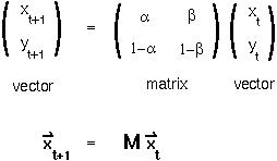
Linear systems of equations like these can also be written in matrix form:

That is, the vector representing the number of methylated and unmethylated sites is written as the product of a matrix times the vector in the previous cell generation.
There are rules of linear algebra that can help us solve this set of linear equations as well as any other set of linear equations.
First we have to review some basics of linear algebra.


A ROW VECTOR has elements arranged left to right, e.g.:

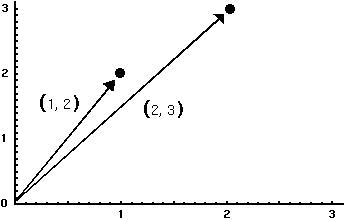
The number of elements in the vector indicates its DIMENSIONALITY. For instance, the (x,y) coordinates drawn on a plane are in 2-dimensions:

An m by n MATRIX has m rows and n columns, e.g.:

(The last example is a special type of matrix known as an IDENTITY matrix, with 1's on the diagonal and 0's everywhere else.)
We will write matrices in boldface (eg A) and vectors with an arrow on top (eg  ).
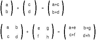
).


Qualification: The vectors (or matrices) added together must have the same dimensionality.
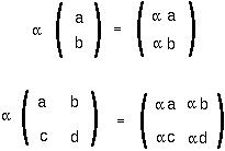
Vector and matrix MULTIPLICATION by a scalar (which may be a constant, a variable or a function but is not a matrix or a vector) is also straightforward:

Vector and matrix MULTIPLICATION is a bit more tricky, but is based on the fact that a row vector times a column vector is equal to the sum:


To multiply a matrix by a matrix, this procedure is then repeated first for the first column of the second matrix and then for the second column of the second matrix, etc:

Qualification: The m by n matrix A can be multiplied on the right by B ONLY if B is an n by p matrix. The resulting matrix will then be an m by p matrix.
Notice that matrix multiplication is not commutative. That is, AB does not generally equal BA. On the other hand, matrix multiplication does satisfy the following laws:


The DETERMINANT of a 2x2 matrix is:

We denote the determinant of matrix A by putting bars around it: |A|. Notice that the determinant of a matrix is a SCALAR (ie not a matrix anymore but just a number or a function). The DETERMINANT of a 3x3 matrix is:

The DETERMINANT of an nxn matrix is obtained by taking the first row and multiplying the first element of the first row by the determinant of the matrix created by deleting the first row and first column MINUS the second element of the first row times the determinant of the matrix created by deleting the first row and second column, etc:

A square mxm matrix A is INVERTIBLE if it may be multiplied by another matrix to get the identity matrix. We call this second matrix the INVERSE of the first:

There are rules to find the inverse of a matrix, one of which is just to ask Mathematica, but for a 2x2 table you should memorize the inverse:
