Methods of Analysis. III. Stability

Global stability is more difficult to determine than local stability.

In the next few lectures, we will see that some of the equations we have been studying may be solved directly, providing a general solution for how the system behaves over time. This general solution can be used to determine the global stability properties of equilibria.

Other methods exist to determine global behavior of the dynamics.

For one-variable discrete models, a graphical method is particularly useful:

Method:

• Plot the function p[t+1] against p[t]
• Note that on the diagonal p[t+1]=p[t]. The function will therefore cross the diagonal ONLY at equilibrium points.
• From the local stability analysis, obtain the slope of the function near the equilibria.
• When the function is above the diagonal, p[t] increases over time.
• When the function is below the diagonal, p[t] decreases over time.

We will demonstrate the method using the diploid selection model.

Methods of Analysis. III. Stability

For the diploid selection model, there are four cases that we must consider.

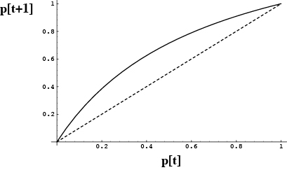
Case 1: Directional selection favoring A (W_AA>W_Aa>W_aa)

The only equilibria are =0 and =1 (the polymorphic equilibrium is not valid in this case).

Near =0, f'()=W_Aa/W_aa and is greater than one.

Near =1, f'()=W_Aa/W_AA and is less than one.

Consequently, the function p[t+1] versus p[t] will look like:

Since this is always above the diagonal, the A allele frequency increases over time.

=1 is globally stable.

Methods of Analysis. III. Stability

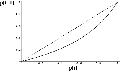
Case 2: Directional selection favoring a (W_AA < W_Aa < W_aa)

The only equilibria are =0 and =1 (the polymorphic equilibrium is not valid in this case).

Near =0, f'()=W_Aa/W_aa and is less than one.

Near =1, f'()=W_Aa/W_AA and is greater than one.

Consequently, the function p[t+1] versus p[t] will look like:

Since this is always below the diagonal, the A allele frequency decreases over time.

=0 is globally stable.

Methods of Analysis. III. Stability

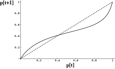
Case 3: Heterozygote Advantage (W_AA < W_Aa > W_aa)

There are now three valid equilibria.

Near =0, f'()=W_Aa/W_aa and is greater than one.

Near the polymorphic equilibrium, f'() is less than one.

Near =1, f'()=W_Aa/W_AA and is greater than one.

Consequently, the function p[t+1] versus p[t] will look like:

This function is above the diagonal when p[t] is less than and the A allele rises in frequency.

This function is below the diagonal when p[t] is greater than and the A allele decreases in frequency.

The polymorphic equilibrium is globally stable.

Methods of Analysis. III. Stability

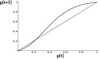
Case 4: Heterozygote Disadvantage (W_AA > W_Aa < W_aa)

There are again three valid equilibria.

Near =0, f'()=W_Aa/W_aa and is less than one.

Near the polymorphic equilibrium, f'() is greater than one.

Near =1, f'()=W_Aa/W_AA and is less than one.

Consequently, the function p[t+1] versus p[t] will look like:

This function is below the diagonal when p[t] is less than and the A allele decreases in frequency.

This function is above the diagonal when p[t] is greater than and the A allele increases in frequency.

There is no single global equilibrium point.

The population will move towards =0 if it starts below the equilibrium and towards =1 if it starts above it.

Back to biology 301 home page.